What's new

The most recent additions, newest first. Each links to the page that covers it in full. In plain terms: every entry is a feature or a fix that is now in Diokle, and the link leads to the page that explains it.

#MSL: 488 of 534 examples match the reference results

Up from 445. Fixes span the whole library:

• Events: one event iteration solves the relations together with the equations they switch, at fixed pre(), after the when-clauses fire; relations inside their hysteresis band keep their value, and cycling modes are resolved by a mode search. This ends the chattering of stuck clutches, brakes, lossy gears, bearing friction and tank overflows.
• Solvers: each state's absolute tolerance is tolerance * |nominal|; a Newton solve that stalls on a fold of a piecewise-linear characteristic searches for a sign change; BDF no longer fails on a first step below the time resolution.
• State selection: reinit(x, ...) makes x a state (stateSelect = always), alias classes keep the declared stateSelect of their members, and stateSelect = prefer wins over default choices (machine currents, spring-damper states).
• Language: final modifiers from outer modifications, redeclared records and model modifiers, constraining-clause modifiers, functions nested in functions, records built from arrays of records, event clocks that tick at initialization, run-time index slices in algorithms, and minimum-norm least squares (dgelsy).

See the scoreboard and Modelica Standard Library.

#Embedded C code and processor in the loop

daedalus codegen-c turns a controller block into portable, allocation-free C99 that steps it at a fixed rate, and daedalus hil closes the loop between that code and a plant simulated by Diokle: on your computer, on an Arduino Uno emulated in simavr, on an ESP32 emulated in QEMU, or on a real board over its serial port. CI runs the whole ladder on every change. daedalus autotune tunes the controller's gains on the closed loop against a step-response specification first. See Embedded C and processor in the loop.

#Scientific machine learning

daedalus.sciml finds the physics a model is missing from measured data, turns it into a formula by sparse regression, and learns neural surrogates that export back to Modelica (and from there to embedded C), in NumPy only. See Scientific machine learning.

#Linear analysis

daedalus linear-analysis and the Linear tab: poles and zeros, Bode and Nyquist plots with margins, step and impulse responses, PID suggestions, balanced truncation and LQR, straight from a Modelica model. See Linear analysis.

#Live plots and dashboards

Results stream into the plot while a simulation runs. Dashboards of sliders, gauges and mini plots change parameters mid-run without restarting. Plots gain matrix layouts, expressions, FFTs, statistics and a plot strip under the diagram. See Live plots and dashboards.

#Equation and initialization debugger

daedalus debug and the Structure tab's Transformation chain and Initialization cards show how a variable is computed and why initialization fails. They find the smallest under- or over-determined set of equations and the components left unconnected. See Equation and initialization debugger.

#Unit checking and display units

Every equation's units are checked and missing units are inferred, with no false alarms on the MSL examples. Plots can show any axis in any compatible unit, or switch to Imperial. See Unit checking.

#Text editor with go-to-definition, completion and rename

The Text view now uses the compiler's own name lookup: F12 to go to a definition, Shift+F12 for usages, F2 to rename, completion, hover and an outline. See Text editor.

#Libraries, packages, diff and parameter data

daedalus lib installs open libraries such as Buildings, ThermoSysPro and OpenIPSL by name and checks uses versions. package zips a model with its resources, diff compares classes structurally (with a diagram view in the workbench), and params-from turns CSV or SSV parameter data into modifiers with unit conversion. See Libraries and packages.

#FMI 3.0 export, FMU and SSP import

daedalus fmu --fmi-version 3 exports FMI 3.0 with exact directional derivatives. FMUs from other tools, FMI 2.0 or 3.0, simulate on their own or as components of a Modelica model, and SSP systems run, import and export. See FMI and SSP.

#Adjoint gradients and design of experiments

sensitivity --adjoint gives the gradient of one quantity with respect to many parameters for about the cost of one extra solve, and drives the L-BFGS-B optimizer (optimize --algorithm lbfgsb; Nelder–Mead is the default). calibrate takes Levenberg–Marquardt steps, with its Jacobian from sensitivities; --optimizer lbfgsb switches to adjoint gradients. daedalus doe runs full, fractional, central composite, Box–Behnken and Latin hypercube designs and fits response surfaces. See Sensitivity, DOE and calibration.

#State machines

The state machines of Modelica 3.6 chapter 17 now translate and simulate: transition, initialState, activeState, ticksInState() and timeInState(), with immediate and delayed transitions, priorities, synchronize, hierarchy, parallel machines and resets. The example from ModelicaReference.StateMachines runs as written. See State machines.

#MSL external C functions and exact lookup tables

The C libraries the MSL calls (ModelicaRandom, ModelicaFFT, ModelicaIO, ModelicaInternal and ModelicaStrings) now have native implementations that run in the browser too. Lookup tables follow the C tables exactly, including CombiTable2D and tables read from files. 21 more MSL examples now match their reference results, among them all the Blocks.Examples.Noise models, the FFT examples and Utilities' matrix file examples. See Modelica Standard Library.

#Structure explorer and state selection

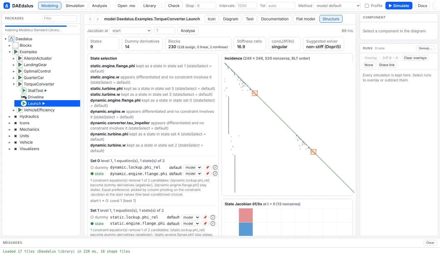
The new Structure tab and daedalus structure show the BLT blocks, the incidence matrix, why each state was chosen, and the state Jacobian's eigenvalues and stiffness. States can be pinned or forbidden there, or with --state NAME=prefer on any command, without editing the model, and a check along the run warns when a static choice breaks down. See Structure and state selection.

#Radau, ESDIRK and automatic switching

Two more stiff solvers, Radau IIA (order 5) and ESDIRK (order 4), and auto, which switches between Dopri5 and BDF as the model turns stiff and back. The implicit methods use an exact Jacobian from the compiled model, and the workbench recommends another method when a run's statistics show it is using the wrong kind. See Solvers.

#Sensitivity, uncertainty, calibration and optimization

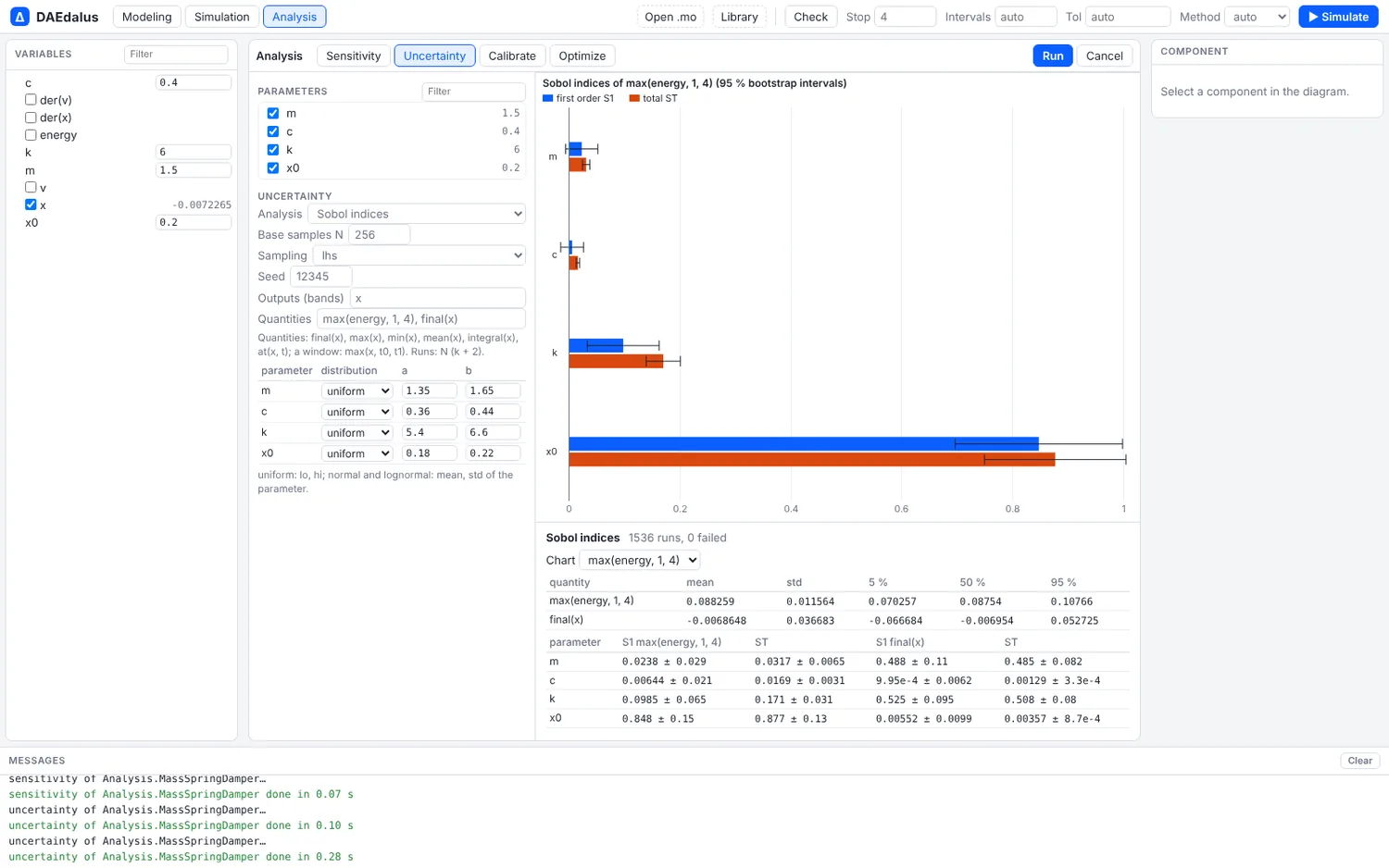
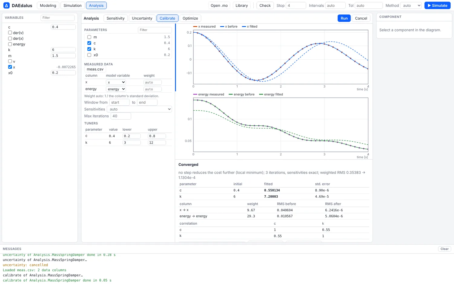
The Analysis mode and daedalus sensitivity | montecarlo | gsa | calibrate | optimize: exact sensitivities, Monte Carlo prediction bands, Sobol and Morris indices, fitting parameters to measured data with standard errors, and design optimization. See Sensitivity and calibration.

#Experiments, sweeps and share links

Every simulation is kept in the Runs pane to overlay or subtract, Sweep… runs a parameter grid on all cores in the browser, daedalus sweep does the same on the command line, and Share link copies an address that reruns the experiment. See Experiments and sweeps.

#Performance analyzer

Profile (or --profile) records the step sizes, the states that limit them, the time in each algebraic loop, the event log and chattering relations, with hints in plain language. See Performance analyzer.

#Graphical editing

The Diagram view is now an editor for your own models: drag components in, connect them, rotate, flip and set parameters, with undo. Edits change only the text they must. See Workbench.

#AI assistant and MCP server

✦ Assistant in the workbench is a chat, via OpenRouter, that can read, write, check and simulate models and read the structure and profile reports, with your own API key. daedalus mcp gives Claude Code and other MCP clients the same tools. See AI assistant and MCP.

#MSL accuracy scoreboard

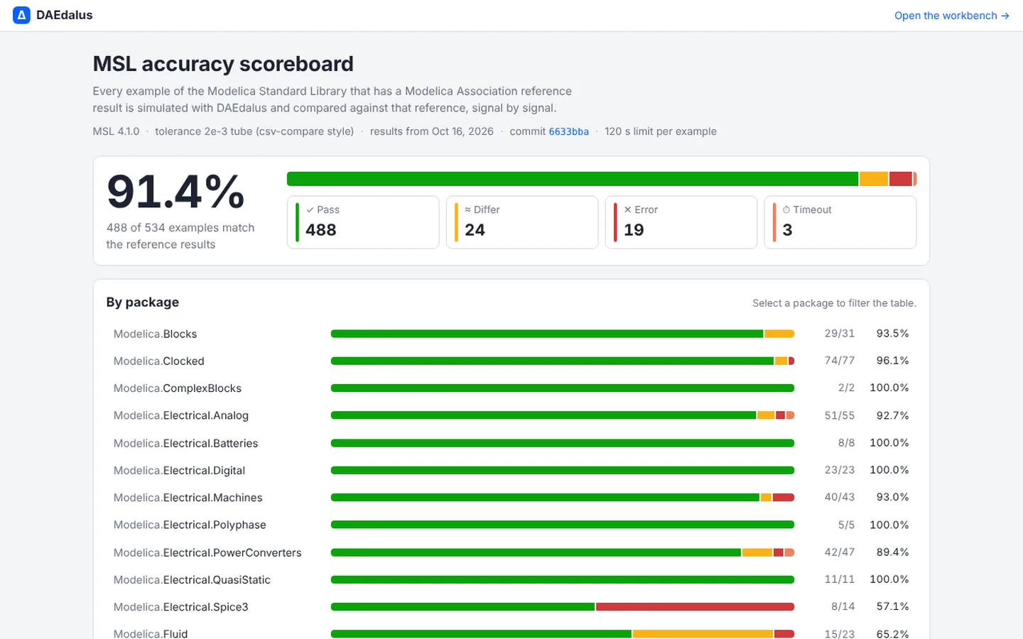
The scoreboard compares every MSL 4.1.0 example with the Modelica Association's reference results, signal by signal: 488 of 534 match, 24 run but differ somewhere, 19 fail and 3 hit the time limit. It breaks the results down by package, shows the signals that differ and the error text for each model, and links each example to the workbench.

See Modelica Standard Library.

#Python API

The daedalus Python package (crates/daedalus-py, built with maturin) runs the compiler in-process, with no server and no licence: load a model, change parameters, simulate to NumPy arrays or pandas, linearize and export FMUs.

import daedalus

m = daedalus.Model("library/Daedalus", "Daedalus.Examples.TorqueConverter.StallTest")
m.set_parameters({"engine.J": 0.3})
r = m.simulate(stop=2.0, vars=["rpm_engine"])
r.time, r["rpm_engine"]

See Python API, which also maps OMPython and Dymola calls onto it.

#.mos scripts, steady states and trim

daedalus run script.mos runs Dymola and OpenModelica regression scripts: loadModel, simulateModel, simulate, simulateExtendedModel, linearizeModel, val, loops and conditionals. daedalus steady finds equilibria with an exact Jacobian and reports their stability, and with --free and --target it trims, for example the input that holds an output at a set value. See Scripts and steady states.

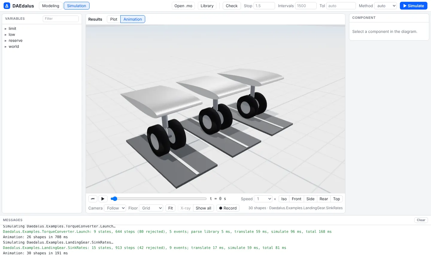
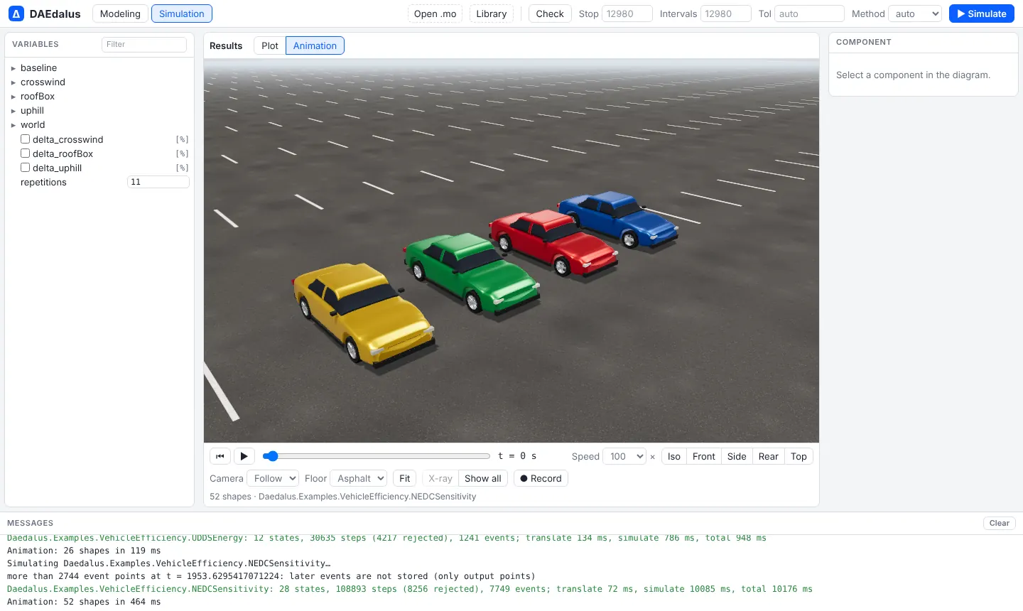
#3-D animation for every example

After Simulate, models with shapes open in the new Animation view: a WebGL scene with studio lighting, camera presets, follow and chase cameras, X-ray selection and WebM recording. It draws every Modelica.Mechanics.MultiBody shape in a result, including STL and OBJ meshes, and the bundled examples got their own visuals through Daedalus.Visualizers: cars that drive the cycles side by side, the landing gear dropping onto the runway, the aileron turning on its hinge.

See 3-D animation.

#Multibody suspensions, rigs and a full car

library/MultiBodyVehicle builds vehicle models on Modelica.Mechanics.MultiBody: double-wishbone, pushrod, multilink and MacPherson corners, an anti-roll bar, a tyre with lift-off, wheel pads and aero loaders, and a 6-DOF car. Nine examples cover suspension kinematics, a K&C rig, a seven-post rig, step steer, lane change and a one-sided bump, and all nine match OpenModelica 1.26.1 to within 0.04 % of each signal's range while running several times faster.

See Multibody vehicles.

#Back and forward between classes

Every class you open is a browser history entry with its own address (/#Package.Model), so Back and Forward, Alt+← and Alt+→, mouse side buttons and the arrows next to the class name walk through them, and a link opens a class directly. The workbench colours now follow the light or dark system theme everywhere, diagrams included. See Workbench.

#Release binaries

Pushing a version tag builds and publishes a GitHub Release with the CLI, the FMI runtime and the example library for Linux, macOS (Apple Silicon and Intel) and Windows, plus the daedalus-casadi Python wheel. See Getting started.

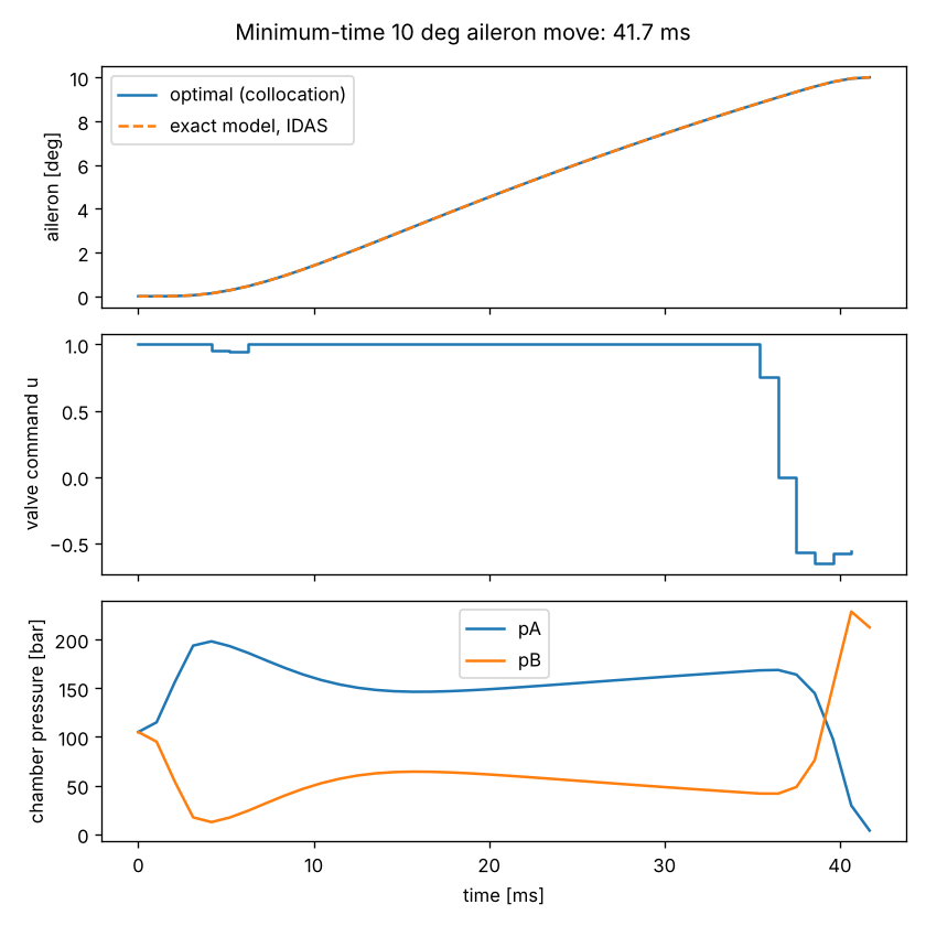
#Optimal control, MPC and estimation with CasADi

daedalus export-casadi hands the index-reduced DAE to CasADi, and the daedalus_casadi Python package solves optimal control problems by direct collocation, runs model predictive control and estimates states and parameters with moving horizon estimation, all referring to model variables by their Modelica names.

See Optimal control.

#Modelica Standard Library 4.1.0 in the browser

The workbench loads MSL 4.1.0 (Modelica, ModelicaServices, Complex) out of the box. The package browser lists all of it within seconds, and a class is parsed only when it is opened or simulated. A nightly job compares every MSL example with the Modelica Association's reference results. See Modelica Standard Library.

#Linearization

daedalus linearize gives the exact state-space matrices A, B, C and D around the initial point or after simulating to a time, as text, JSON or an OpenModelica-style linearized_model. See Linearization.

#FMI 2.0 export

daedalus fmu writes one FMU with both Model Exchange and Co-Simulation, validated with FMPy in CI. See FMI 2.0 export.

#Multibody closed loops

Planar kinematic loops on a free body, driven loops and steady-state initialization now work, which is what the suspension models above are built on.

The longer-term plan is in the Roadmap.