Optimal control, MPC and estimation with CasADi
Diokle can hand any model it translates to CasADi,
the open-source framework for nonlinear optimization and optimal control. On top
of that, the daedalus_casadi Python package (in python/) solves three kinds
of problem:
- optimal control problems (OCP), such as a minimum-time move;
- model predictive control (MPC): an OCP re-solved in a closed loop;
- moving horizon estimation (MHE) of states and parameters from measurements.
In plain terms: you say what you want, such as reaching a target as fast as possible or keeping an error small, and the optimizer finds the inputs that achieve it. MPC repeats that search at every step using fresh measurements. MHE runs the other way: it estimates the hidden states and parameters from what was measured.
The model stays in Modelica. Inputs that the optimizer may choose are
top-level input variables, and every other model variable can appear in a
cost or a constraint by its name.
How it works
.mo ──► Diokle frontend + backend ──► daedalus export-casadi ──► JSON ──► daedalus_casadi ──► CasADi / IPOPT
        (alias elimination, index                                            (SX expressions,
         reduction, BLT, tearing)                                             direct collocation)
daedalus export-casadi writes the model as Diokle compiles it for
simulation. That is a semi-explicit DAE of index 1:
der(x) = f(t, x, z, u, p)
0 = g(t, x, z, u, p)| Symbol | What it holds |
|---|---|
x |
The states Diokle selected, including dummy-derivative state selection after index reduction. |
z |
The tearing variables of the algebraic loops. Models without loops have no z: the problem is a plain ODE. |
u |
Top-level input variables. |
p |
Public parameters with a literal value. These are the ones a user can change. Other parameters are expressions of them. |
The hard symbolic work therefore happens before CasADi sees the model:
- alias elimination;
- Pantelides index reduction;
- BLT sorting and tearing.
The optimizer gets a small, well-posed system. For example, the hydraulic aileron actuator has 6 states and 2 algebraic unknowns, out of a few hundred flat equations.
The JSON document also holds the value of every variable after Diokle' own
initialization. These values give a consistent initial state, and guesses for
z, even when the model initializes from steady-state initial equations.
Conversions.
- Event relations become
if_elseexpressions. - Tables become piecewise polynomials with the same interpolation and extrapolation as the simulator.
when-clauses are not part of a continuous optimization problem. They are left out with a warning. Discrete variables, andpre()of non-continuous variables, keep their initial values.delay(), clocked equations and functions withwhile-loops are reported as unsupported.
Setup
cargo build --release                  # builds target/release/daedalus
pip install casadi numpy matplotlib    # matplotlib only for the example plots
The package is plain Python. Either:
- run the examples from the repository;
- add
python/toPYTHONPATH; - or install it with
pip install -e python.
It finds the daedalus executable in this order:
$DAEDALUS_BIN;PATH;target/releaseof the checkout.
Export
From the command line:
./target/release/daedalus export-casadi library/Daedalus \
    -m Daedalus.Examples.OptimalControl.AileronServo -o servo.json [-p name=value ...]
From Python:
import daedalus_casadi as dc

m = dc.export("Daedalus.Examples.OptimalControl.AileronServo")   # or dc.load("servo.json")
m.x_names, m.z_names, m.u_names, m.p_names
m.ode, m.alg                 # casadi.SX in m.t, m.x, m.z, m.u, m.p
m["delta_deg"]               # any variable as an expression of t, x, z, u, p
m.x0, m.z0, m.u0, m.p0       # values after Diokle' initialization
m.dae_function()             # Function(t, x, z, u, p) -> (ode, alg)
m.jacobians()                # linearization (A, B), with z eliminated
dc.simulate(m, t_grid, u=..) # CasADi IDAS / CVODES, inputs held per intervalOptimal control
The problem in symbols. An optimal control problem chooses the inputs (and the free end time , if asked) that minimize a cost while the model and the limits hold:
A minimum-time move has and a free : the optimizer finds the shortest time that reaches the target. Collocation turns the continuous problem into a large but sparse nonlinear program, which IPOPT solves.
dc.OCP transcribes the model by direct collocation:
- inputs are constant on each interval;
- states follow polynomials through Radau IIA points, which are stiffly accurate and suit DAEs;
- algebraic variables are unknowns at every collocation and mesh point.
Unknowns are scaled by each variable's nominal attribute or initial magnitude.
IPOPT then sees numbers of order one, even for pressures in pascal.
ocp = dc.OCP(m, N=40, free_time=True, T_guess=0.06)   # or T=0.1 for a fixed horizon
ocp.bound("u", -1, 1)                                  # inputs, or any variable on the mesh
ocp.subject_to(ocp.final("delta_deg") == 10, ocp.final("aileron.w") == 0)
ocp.minimize(ocp.T)                                    # or ocp.integral(m["..."]**2), ...
ocp.guess(dc.simulate(m, t_grid, u=feedback_law))      # optional initial guess
sol = ocp.solve()
sol.T, sol.t, sol.u, sol["act.cylinder.pA"]
The building blocks are:
ocp.at(name, k),ocp.initial(name),ocp.final(name),ocp.trajectory(name);ocp.integral(expr), by the collocation quadrature;ocp.input(name).
ocp.opti is the underlying casadi.Opti, for anything else.
free_params=[...] turns parameters into decision variables, for design
optimization or parameter estimation.
Kinks. Saturations, dead zones and valve metering edges are min/max/abs
in the model. An optimum often sits exactly on such a kink, for example a valve
held at zero opening, and IPOPT then fails to converge.
dc.export(..., smooth=1e-3) replaces those kinks by smooth approximations of
that width. smooth_if=True also blends the branches of if a < b expressions.
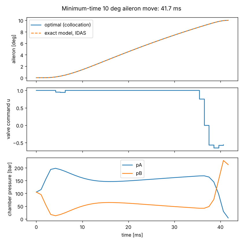
The aileron example solves on the smoothed model, then replays the optimal
command on the exact model to show the difference is negligible.
Model predictive control
At every sampling instant the controller takes the measured state , solves the optimal control problem over the next seconds, and applies only the first piece of the answer. Then it measures again and solves again. This receding horizon is what makes MPC robust: a disturbance is corrected at the next step, not at the end of a fixed plan.
mpc = dc.MPC(m, N=25, dt=0.01, degree=2)
o = mpc.ocp
mpc.bound("F_act", -2500, 2500)
mpc.minimize(o.integral(m["a_body"]**2) + 10*o.integral((m["travel"]/0.03)**2)
             + o.integral((m["F_act"]/2500)**2))
u0 = mpc.step(x_measured, t)          # one solve, warm-started from the previous one
closed_loop = mpc.run(t_end=1.0)      # closed loop against the model (or plant=...)
The initial state and start time are parameters of one NLP that is built once.
Each step warm-starts from the previous solution, shifted by one interval.
Time-varying model inputs, such as a road profile given as a function of
time, are therefore previewed by the prediction.
Moving horizon estimation
The estimator is the mirror image of MPC: it looks back over a window of the last intervals and finds the states and parameters that best explain the measurements. Its objective is a weighted least-squares fit,
where and are the prior estimates (the arrival cost), are process disturbances, and , , are weights set from standard deviations in each variable's own units. After each window the prior moves to the new estimate, one interval later.
mhe = dc.MHE(m, N=30, dt=1.0, measurements=["v_kmh"], meas_std=[0.3],
             process_std=[1e-3, 0.05], estimate_params=["body.Cd", "body.crr"],
             param_prior_std=[0.01, 0.001])
x_end, p_est = mhe.step(y_window, t0)       # y_window: (N + 1) x n_measurements
t_est, x_est, p_est = mhe.run(t, y)         # one window per new sample
Each window is a weighted least-squares problem over:
- the initial state;
- a disturbance on the state at every mesh point;
- the chosen parameters.
It is constrained by the model, with an arrival cost that carries the previous
estimate forward. Known inputs are passed with u=.
Examples
The plants are in Daedalus.Examples.OptimalControl. The scripts are in
python/examples/, and each takes --plot out.png.
| Script | Plant | Problem | Result |
|---|---|---|---|
ocp_aileron.py |
AileronServo: 3000 psi supply, servo valve, cylinder, aileron with hinge moment; valve command u ∈ [-1, 1] |
Fastest 10° deflection that ends at rest | 41.7 ms, full-open then a reverse braking pulse; 42 IPOPT iterations, about 1 s |
mpc_active_suspension.py |
ActiveSuspension: quarter car, soft damper, force actuator F_act |
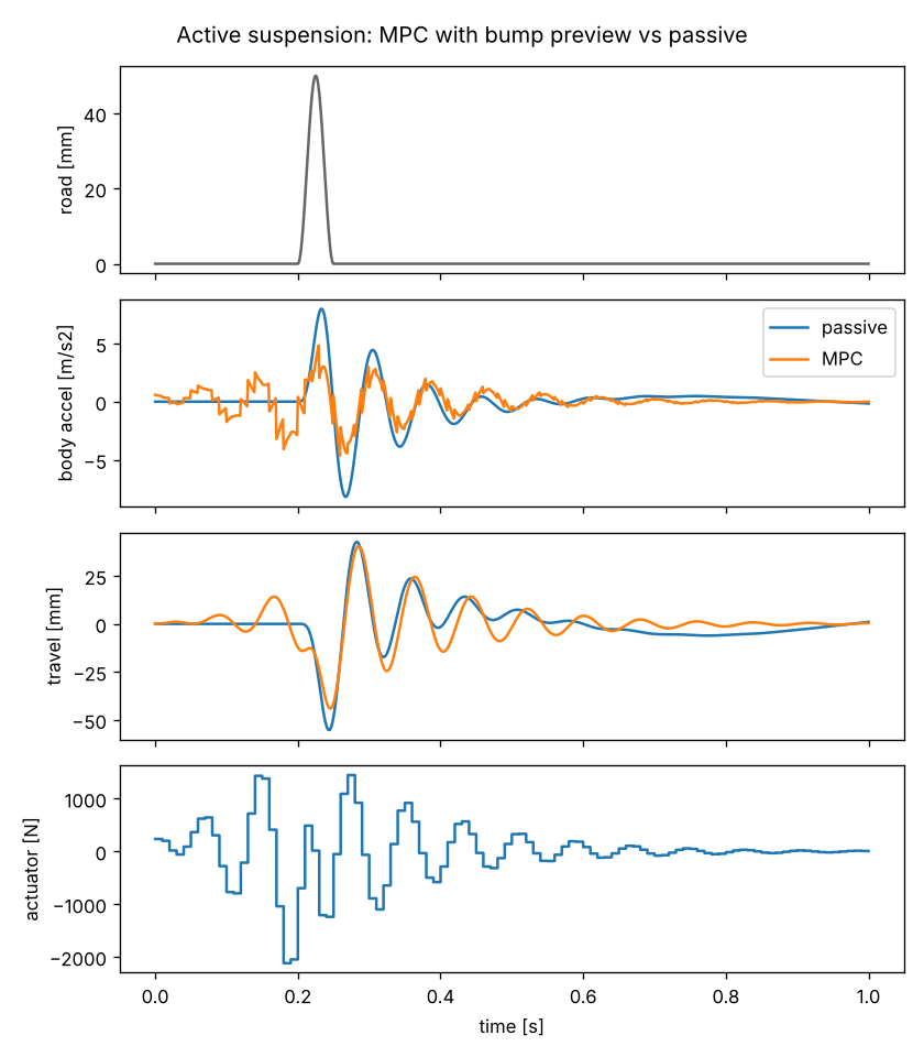
MPC every 10 ms over a 0.25 s horizon that previews a 50 mm bump | Body acceleration −35 % rms and −41 % peak, suspension travel −20 % against the passive car; median solve 23 ms |
mhe_coastdown.py |
CoastDownTest: a 1650 kg car coasting from 130 km/h |
Estimate speed, Cd and crr from speed readings with 0.3 km/h noise |
Cd 0.331 (true 0.33), crr 0.0119 (true 0.012), speed error 0.06 km/h rms |
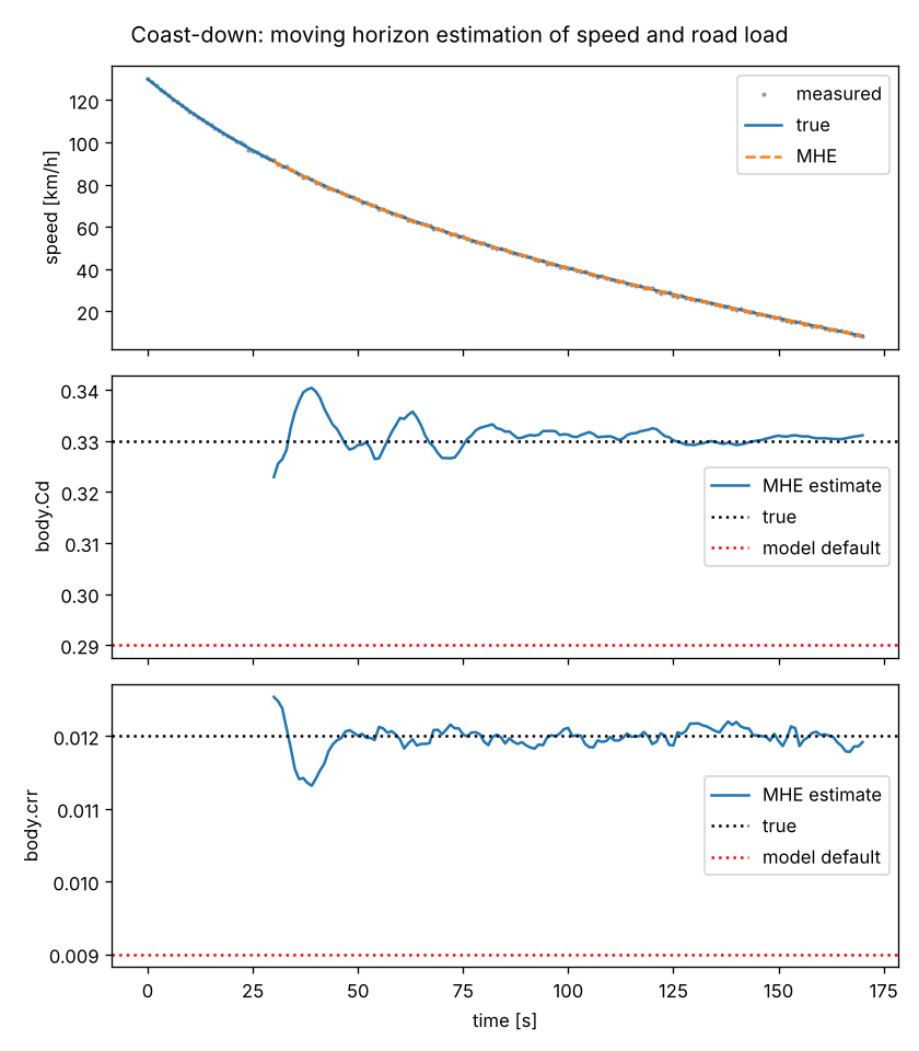
The MHE measurements come from Diokle itself, which simulates the "real" car with different coefficients from those of the model being estimated.
The numbers were measured on a 4-core cloud container with CasADi 3.8 and IPOPT with MUMPS.
Tests
cargo test --release -p daedalus-core --test library casadi
python -m pytest python/tests
The Python tests check four things:
- every exported variable evaluates to Diokle' initialized value;
- CasADi simulations of the exported models match Diokle simulations;
- tables interpolate as in the simulator;
- each of the three problems reaches its expected result.