Linear analysis

daedalus linear-analysis and the workbench's Linear tab linearize a model around an operating point and analyze its input-output pairs. You get poles and zeros, Bode and Nyquist plots with margins, and step and impulse responses. It also suggests PID settings, reduces the model by balanced truncation and computes an LQR gain. It is the classical control toolbox, applied directly to the Modelica model.

Linear view of OptimalControl.ActiveSuspension: Bode plot of a_body from F_act, pole-zero map, step response and the summary with margins and poles

What it computes

For the chosen inputs and outputs, after linearizing like linearize at the start or after simulating to --at T:

poles, with natural frequency and damping, and whether the model is stable;
per input → output pair:
- transmission zeros, DC gain and relative degree;
- Bode and Nyquist data with gain and phase margins;
- step and impulse responses with rise time, settling time and overshoot;
- PID suggestions: SIMC PI and Ziegler–Nichols PID, from a first-order-plus-dead-time fit of the step response;
--reduce N: balanced truncation to N states, with the Hankel singular values, the H∞ error bound and the reduced model's responses for comparison;
--lqr q,r: the LQR gain for Q = q·I, R = r·I, with its closed-loop poles.

Outputs can be any continuous variable or state, not only top-level outputs.

The Linear tab for OptimalControl.ActiveSuspension in the workbench: Bode magnitude and phase, pole-zero map, step response and the summary with margins and the PID suggestion

The math in brief

Near the operating point the model is a linear state-space system,

\dot{x} = A\,x + B\,u, \qquad y = C\,x + D\,u

and each input-output pair has the transfer function

G(s) = C\,(sI - A)^{-1} B + D .

Poles are the eigenvalues of $A$ . The model is stable when all of them have a negative real part. A pole $p$ has damping $\zeta = -\operatorname{Re}(p)\,/\,|p|$ .
DC gain is $G(0)$ : the steady change of $y$ for a unit step in $u$ .
Zeros are the values of $s$ where $G(s)$ drops to zero.
Balanced truncation keeps the states that are easiest to excite and to observe. The Hankel singular values $\sigma_i$ rank them, and the error of the reduced model is bounded by $\|G - G_r\|_\infty \le 2\sum_{i > r}\sigma_i$ .

Step response and PID suggestions

Each step response is fitted with a first-order model plus dead time,

G(s) \approx \frac{K\,e^{-Ls}}{\tau\,s + 1},

using Smith's two-point method. The times $t_{28}$ and $t_{63}$ at which the response reaches 28.3 % and 63.2 % of its final value give $\tau = 1.5\,(t_{63} - t_{28})$ and $L = t_{63} - \tau$ . From that fit:

SIMC PI (Skogestad), with closed-loop time constant $\tau_c = \max(L,\ 0.1\,\tau)$ :

$K_p = \frac{\tau}{K\,(\tau_c + L)}, \qquad T_i = \min\bigl(\tau,\ 4\,(\tau_c + L)\bigr)$
Ziegler–Nichols reaction-curve PID, only when there is dead time:

$K_p = \frac{1.2\,\tau}{K\,L}, \qquad T_i = 2L, \qquad T_d = 0.5\,L$

A first-order fit is rough when the response overshoots. The tool says so, and the gains are a starting point to check by simulation.

LQR gain

--lqr q,r minimizes the cost

J = \int_0^\infty \left( x^T Q\,x + u^T R\,u \right) dt, \qquad Q = q\,I,\quad R = r\,I,

over the feedback law $u = -Kx$ , with $K = R^{-1} B^T P$ . The matrix $P$ solves the algebraic Riccati equation

A^T P + P A - P\,B\,R^{-1} B^T P + Q = 0 .

The closed-loop poles are the eigenvalues of $A - BK$ . Small $r$ compared with $q$ means cheap control: the gain is large and the poles move far to the left.

Example: an active suspension

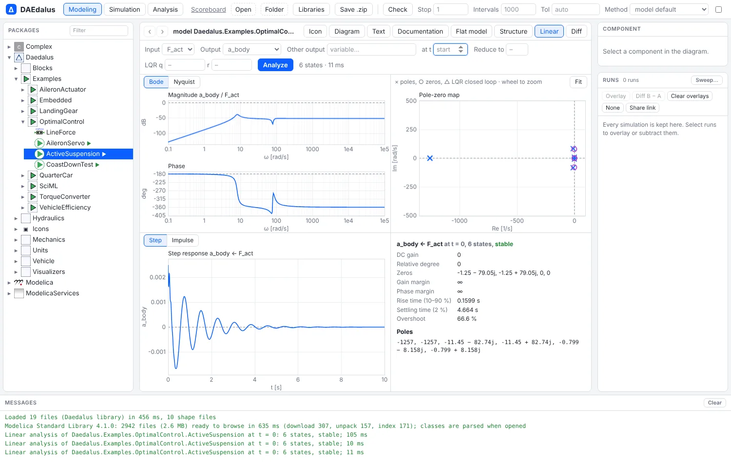
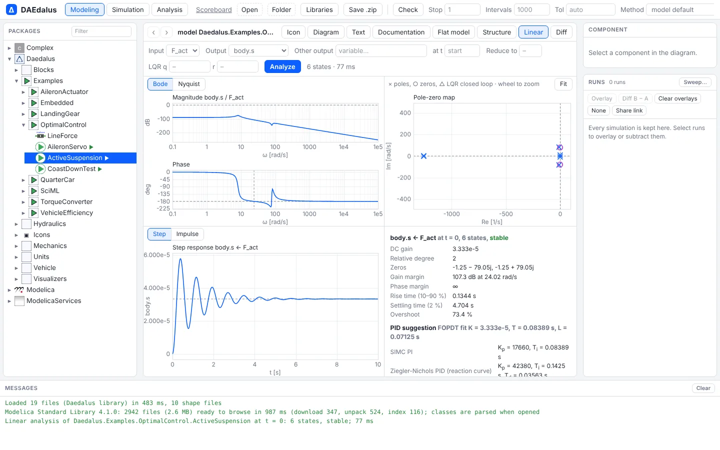
Daedalus.Examples.OptimalControl.ActiveSuspension is a quarter car with an actuator force F_act between body and wheel. How do body acceleration and suspension travel respond to it?

daedalus linear-analysis library/Daedalus -m Daedalus.Examples.OptimalControl.ActiveSuspension \
    --inputs F_act --outputs a_body,travel --reduce 2 --lqr 1,1e-6

linear analysis of Daedalus.Examples.OptimalControl.ActiveSuspension at t = 0 (6 states, 1 inputs, 2 outputs)

poles (stable):
  -1.256637e3                          |p| = 1.2566e3 rad/s, damping 1.000
  -1.256637e3                          |p| = 1.2566e3 rad/s, damping 1.000
  -1.145095e1 - 8.273502e1i            |p| = 8.3524e1 rad/s, damping 0.137
  -1.145095e1 + 8.273502e1i            |p| = 8.3524e1 rad/s, damping 0.137
  -7.990487e-1 - 8.158075e0i           |p| = 8.1971e0 rad/s, damping 0.097
  -7.990487e-1 + 8.158075e0i           |p| = 8.1971e0 rad/s, damping 0.097

F_act -> travel:
  DC gain        3.333e-5
  rel. degree    2 (high-frequency gain 2.7500e-2)
  zeros:
    -1.136364e-1 - 2.383629e1i
    -1.136364e-1 + 2.383629e1i
  step: rise 0.1742 s, settling (2 %) 4.684 s, overshoot 65.37 %, peak 5.5123e-5 at 0.3926 s
  FOPDT fit: K = 3.3333e-5, T = 9.7278e-2 s, L = 5.7253e-2 s
  SIMC PI: Kp = 2.5487e4, Ti = 9.7278e-2 s, Td = 0.0000e0 s
  Ziegler-Nichols PID (reaction curve): Kp = 6.1168e4, Ti = 1.1451e-1 s, Td = 2.8626e-2 s
  note: the step response overshoots: a first-order fit is rough, check the loop by simulation

balanced truncation to 2 states:
  Hankel singular values: 6.328e-3 5.226e-3 1.227e-3 1.078e-3 0.000e0 0.000e0
  H-infinity error bound: 4.610e-3
  reduced poles:
    -7.857228e-1 - 8.074004e0i
    -7.857228e-1 + 8.074004e0i

LQR (Q = 1 I, R = 0.000001 I), u = -K x:
  [   -2.3481e3     5.7678e2    -4.3634e2     2.3814e3    -3.1016e3    -1.6380e0]
  closed-loop poles:
    -1.256637e3
    -1.256637e3
    -1.703504e1 - 8.179908e1i
    -1.703504e1 + 8.179908e1i
    -1.390127e0 - 8.079972e0i
    -1.390127e0 + 8.079972e0i

The body mode at 8.2 rad/s (1.3 Hz) is barely damped (ζ = 0.097), and the wheel hop mode sits at 84 rad/s (13 Hz). The two fast real poles at 1257 rad/s are the actuator. Two states keep the body mode, and the LQR gain raises its damping from 0.097 to 0.17.

In the workbench

Open a model and pick the Linear tab of the model view. Choose the inputs and outputs, the operating point (start, or after simulating to a time) and the plot: Bode or Nyquist, the pole-zero map, and the step or impulse response, next to the same summary as the command line.

Output files

A text summary goes to stdout. -o file.json writes everything; -o file.csv writes the Bode data (--bode) and the step responses (--step, to <file>_step.csv):

daedalus linear-analysis model.mo -m MyModel --at 2 --bode --step -o bode.csv

How it is computed

The numerics are in crates/daedalus-core/src/lti.rs, with no extra dependencies:

Bode points cost O(n²) each, after a Householder Hessenberg reduction;
step responses are exact for a step (zero-order hold with the Padé matrix exponential);
Lyapunov and Riccati equations are solved with the matrix sign function;
transmission zeros are the zero-dynamics eigenvalues of a minimal realization of each pair.

Balanced truncation needs a stable model, and the dense algorithms are meant for models with up to a few hundred states. For a fully tuned controller on the closed loop, see daedalus autotune in Embedded C and processor in the loop.

Linear analysis

#What it computes

#The math in brief

#Step response and PID suggestions

#LQR gain

#Example: an active suspension

#In the workbench

#Output files

#How it is computed