Scientific machine learning

daedalus.sciml combines Modelica models with machine learning, in NumPy only:

• Missing physics. Keep the physics you trust in Modelica, give the part you cannot explain a top-level input, and recover that input's values from measurements.
• Sparse regression. Turn the recovered values into a short formula built from a few candidate terms, such as products of the variables (SINDy), and put the formula back into the model as an equation.
• Neural surrogates. Run the model for many parameter values, then train a small neural network that predicts the quantities you care about from those parameters. Export the network as a Modelica block that simulates anywhere and compiles to embedded C.

In short: you keep the equations you trust, and let the data fill in the rest. It needs the Python API and NumPy, nothing else: no PyTorch or JAX, and every network is small enough to train in seconds on a laptop.

#The worked example

Daedalus.Examples.SciML holds a DC motor whose friction is missing from the model. python/examples/sciml_motor.py runs the whole workflow:

data: 2501 samples of speed and current over 5 s, noise 0.01 rad/s
missing torque recovered in 0.28 s: RMS error 2.46e-04 N.m (range 1.79e-02)
sparse regression: tau_missing = 2.00314e-07*w*abs(w) + 0.00399621*tanh(w/2.0)   (R2 0.99813, 2 of 8 terms)
  as Modelica:  MotorKnown m(tau_missing=2e-07*m.w*abs(m.w) + 0.004*tanh(m.w/2.0));
  true law:     4e-3*tanh(w/2) + 2e-7*w*abs(w)
  speed error vs the rig: 0.0017 rad/s with the discovered law, 4.1 rad/s without

neural surrogate in 0.7 s
surrogate of 2 outputs over 2 parameters, 120 runs (24 held out)
  w_peak: R2 1.0000, max error 0.212 (range 31.56)
  i_rms: R2 0.9999, max error 0.01005 (range 1.307)

Timings depend on the machine. The speed check simulates the fitted coefficients at full precision. The Modelica line rounds them to three digits, and MotorDiscovered in the library uses that rounded form. With the fitted law the speed stays within 0.0017 rad/s of the rig over 5 s, against 4.1 rad/s without the friction term.

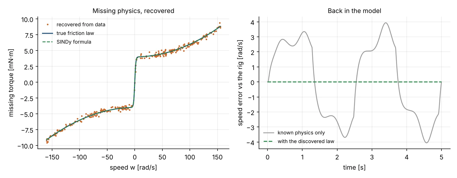
#Missing physics

The known model, with the unknown torque as an input:

model MotorKnown
  parameter Real R=1.2, L=5e-3, k=0.05, J=2e-4, b=1e-5;
  input Real tau_missing "Unknown torque, found from data";
  Real u, i(start=0, fixed=true), w(start=0, fixed=true);
equation
  u = 6*sin(2*pi*0.4*time) + 3*sin(2*pi*1.3*time);
  L*der(i) = u - R*i - k*w;
  J*der(w) = k*i - b*w - tau_missing;
end MotorKnown;

import daedalus
from daedalus import sciml

known = daedalus.Model("library/Daedalus", "Daedalus.Examples.SciML.MotorKnown")
tau = sciml.missing_term(known, t, {"w": w_measured, "i": i_measured}, "tau_missing")

missing_term estimates the time derivatives of the measured states (local polynomial fits, smooth_derivative), then at every sample finds the value of the input for which the model's derivatives match them best. The model's right-hand side comes from Model.derivatives, which evaluates der(x) = f(t, x, u) at any points, so any Modelica model works, with its algebraic loops, tables and events.

This answers the question a universal differential equation answers, by collocation instead of differentiating through the solver: it is fast (thousands of points in a fraction of a second) and needs every state measured. When some states are not measured, fit the parameters of a candidate law with daedalus calibrate instead.

#Symbolic regression

theta, terms = sciml.candidate_library({"w": w_measured}, degree=2, tanh_scales=(0.5, 2.0, 8.0))
fit = sciml.sindy(theta, tau, terms, threshold=0.1)
print(fit.expression(prefix="m.", digits=3))
# 2e-07*m.w*abs(m.w) + 0.004*tanh(m.w/2.0)

candidate_library builds monomials up to a degree and, for friction-like terms, sign(x), x*abs(x) and tanh(x/s); add your own columns as needed. sindy keeps the fewest terms that explain the data (sequentially thresholded least squares on normalised columns, so threshold is relative). The expression is Modelica text, ready for a modifier:

model MotorDiscovered
  MotorKnown m(tau_missing=0.004*tanh(m.w/2.0) + 2e-07*m.w*abs(m.w));
end MotorDiscovered;

#Neural surrogates

truth = daedalus.Model("library/Daedalus", "Daedalus.Examples.SciML.MotorTruth")

def qoi(r):
    return {"w_peak": r["w"].max(), "i_rms": (r["i"] ** 2).mean() ** 0.5}

s = sciml.fit_surrogate(truth, {"Tc": (0, 1e-2), "J": (1e-4, 4e-4)}, qoi, n=120,
                        simulate={"vars": ["w", "i"]})
print(s.report())                 # R2 and largest error on held-out runs
s.predict(Tc=4e-3, J=2e-4)        # {'w_peak': 155.2, 'i_rms': 1.344}
open("MotorSurrogate.mo", "w").write(s.to_modelica("MotorSurrogate"))

fit_surrogate draws a Latin hypercube over the bounds, simulates the runs in parallel threads, holds a fifth of them out, and trains a multilayer perceptron (tanh layers, Adam). qoi is a list of variables (their final values) or a function of the result. The exported block has one input per parameter and one output per quantity, written with scalar equations only, so it runs in any Modelica tool and through daedalus codegen-c on a microcontroller.

For a network trained elsewhere, sciml.MLP can be filled with its weights and exported the same way.

#Reference